Usage example: Euler characteristic surfaces
This notebook provides usage examples for the euchar.surface module.
Euler characteristic surfaces of 2D and 3D images with values sampled from uniform distributions.
Euler characteristic surfaces of finite point sets in \(\mathbb{R}^2\) and \(\mathbb{R}^3\), obtained using bifiltrations resulting from the combination of the Alpha filtration and the filtration induced by an estimate of the density at points.
import numpy as np
import euchar.utils
from euchar.surface import images_2D, images_3D, bifiltration
from euchar.filtrations import alpha_filtration_2D, alpha_filtration_3D, inverse_density_filtration
import matplotlib.pyplot as plt
#plt.style.use("seaborn-whitegrid")
plt.rcParams.update({"font.size": 16})
from seaborn import distplot
Synthetic data
Images
np.random.seed(0)
m = 32
max_intensity = 256

img1_2D = np.random.randint(0, max_intensity, size=(m, m))
img2_2D = np.random.randint(0, max_intensity, size=(m, m))
img1_3D = np.random.randint(0, max_intensity, size=(m, m, m))
img2_3D = np.random.randint(0, max_intensity, size=(m, m, m))
Finite point sets
np.random.seed(0)
N = 100
points_2D = np.random.rand(N, 2)
points_3D = np.random.rand(N, 3)
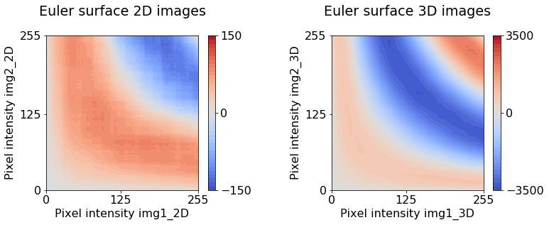
Euler characteristic curves of 2D and 3D image
For the following computation, the vector_2D_changes is
automatically computed by images_2D().
euler_char_surf_2D = images_2D(img1_2D, img2_2D)
To avoid recomputing it every time, it can be passed as a parameter to
images_2D().
Precompute it with
vector_2D_changes = euchar.utils.vector_all_euler_changes_in_2D_images()
For the following computation, the vector of all possible Euler changes in the case of 3D images needs to be precomputed and saved to a file.
For example one could do this by running
vector_3D_changes = euchar.utils.vector_all_euler_changes_in_3D_images()
np.save("vector_3D_changes.npy", vector_3D_changes)
vector_3D_changes = np.load("vector_3d_changes.npy")
euler_char_surf_3D = images_3D(img1_3D, img2_3D, vector_3D_changes)
We can then display the Euler characteristic surfaces as contour plots.
color_map = 'coolwarm'
dx = 0.05
dy = 0.05

domain = np.arange(256)
levels_2D = [int(el) for el in np.linspace(-150, 150, num=40)]
colorbar_ticks_2D = [-150, 0, 150]
levels_3D = [int(el) for el in np.linspace(-3500, 3500, num=40)]
colorbar_ticks_3D = [-3500, 0, 3500]
fig, ax = plt.subplots(1, 2, figsize=(12,4))
plt.subplots_adjust(wspace=0.5)
xx, yy = np.meshgrid(domain, domain)
cmap = plt.get_cmap(color_map)

cf = ax[0].contourf(xx + dx/2., yy + dy/2.,
                    euler_char_surf_2D,
                    levels=levels_2D, cmap=cmap)
fig.colorbar(cf, ax=ax[0], ticks=colorbar_ticks_2D)
ax[0].set(title="Euler surface 2D images\n",
       xticks=[0, 125, 255], yticks=[0, 125, 255],
       xlabel="Pixel intensity img1_2D", ylabel="Pixel intensity img2_2D")

cf = ax[1].contourf(xx + dx/2., yy + dy/2.,
                    euler_char_surf_3D,
                    levels=levels_3D, cmap=cmap)
fig.colorbar(cf, ax=ax[1], ticks=colorbar_ticks_3D)
ax[1].set(title="Euler surface 3D images\n",
       xticks=[0, 125, 255], yticks=[0, 125, 255],
       xlabel="Pixel intensity img1_3D", ylabel="Pixel intensity img2_3D");
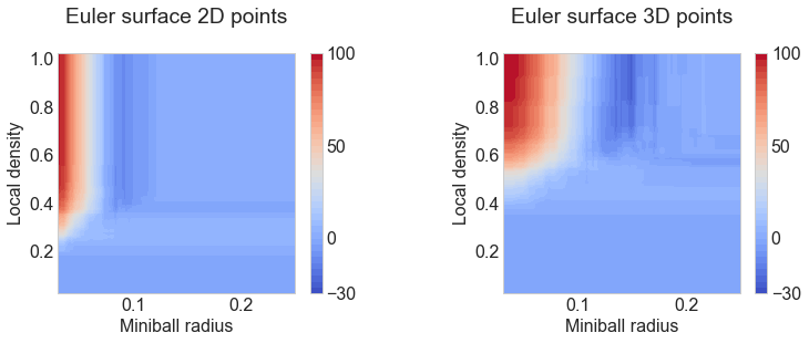
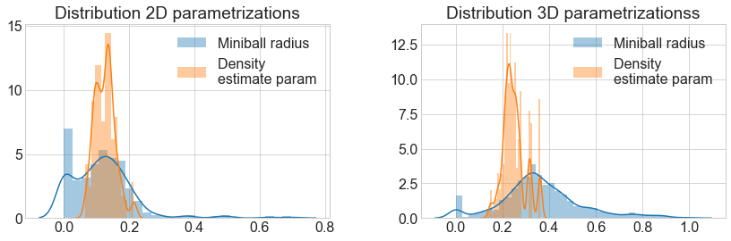
Euler characteristic surfaces of finite point sets
We obtain the bifiltrations in the form of arrays of indices of
points_2D and points_3D.
simplices_2D, miniball_2D = alpha_filtration_2D(points_2D)
density_2D = inverse_density_filtration(points_2D, simplices_2D, n_neighbors=6)
simplices_3D, miniball_3D = alpha_filtration_3D(points_3D)
density_3D = inverse_density_filtration(points_3D, simplices_3D, n_neighbors=6)
plt.style.use("seaborn-whitegrid")
fig, ax = plt.subplots(1, 2, figsize=(14,4))
plt.subplots_adjust(wspace=0.3)
_ = distplot(miniball_2D, label="Miniball radius", ax=ax[0])
_ = distplot(density_2D, label="Density \nestimate param", ax=ax[0])
ax[0].set(title="Distribution 2D parametrizations"); ax[0].legend()
_ = distplot(miniball_3D,  label="Miniball radius", ax=ax[1])
_ = distplot(density_3D, label="Density \nestimate param", ax=ax[1])
ax[1].set(title="Distribution 3D parametrizationss"); ax[1].legend();
We produce arrays bins1_2D, bins2_2D and bins1_3D,
bins2_3D, used to discretize the domains of the distributions of 2D
and 3D parametrizations.
bins1_2D = np.linspace(0.0, 0.4, num=200)
bins2_2D = np.linspace(0.0, 1,  num=200)
bifilt_2D = bifiltration(simplices_2D, density_2D, miniball_2D,
                           bins1_2D, bins2_2D)
bins1_3D = np.linspace(0.0, 0.4,  num=200)
bins2_3D = np.linspace(0.0, 1, num=200)
bifilt_3D = bifiltration(simplices_3D, density_3D, miniball_3D,
                           bins1_3D, bins2_3D)
Again we plot the obtained Euler characteristic surfaces as contour plots.
color_map = 'coolwarm'
dx = 0.05
dy = 0.05

levels_2D = [int(el) for el in np.linspace(-30, 100, num=40)]
colorbar_ticks_2D = [-30, 0, 50, 100]
levels_3D = [int(el) for el in np.linspace(-30, 100, num=40)]
colorbar_ticks_3D = [-30, 0, 50, 100]
fig, ax = plt.subplots(1, 2, figsize=(12,4))
plt.subplots_adjust(wspace=0.5)

cmap = plt.get_cmap(color_map)
xx2, yy2 = np.meshgrid(bins1_2D, bins2_2D)
cf = ax[0].contourf(xx2 + dx/2., yy2 + dy/2.,
                    bifilt_2D,
                    levels=levels_2D, cmap=cmap)
fig.colorbar(cf, ax=ax[0], ticks=colorbar_ticks_2D)
ax[0].set(title="Euler surface 2D points\n",  xlim=[0.03, 0.25],
          xlabel="Miniball radius", ylabel="Local density")

xx3, yy3 = np.meshgrid(bins1_2D, bins2_3D)
cf = ax[1].contourf(xx3 + dx/2., yy3 + dy/2.,
                    bifilt_3D,
                    levels=levels_3D, cmap=cmap)
fig.colorbar(cf, ax=ax[1], ticks=colorbar_ticks_3D)
ax[1].set(title="Euler surface 3D points\n", xlim=[0.03, 0.25],
          xlabel="Miniball radius", ylabel="Local density");